
Axial Tomography in Live Cell Microscopy


1
Institute of Applied Research, Aalen University, 73430 Aalen, Germany
2
Kirchhoff-Institute for Physics, University Heidelberg, 69120 Heidelberg, Germany
3
Max Planck Institute for Polymer Research, 55128 Mainz, Germany
4
Institute of Molecular Biology (IMB), 55128 Mainz, Germany
*
Author to whom correspondence should be addressed.
Biophysica 2024, 4(2), 142-157; https://doi.org/10.3390/biophysica4020010
Submission received: 25 January 2024
/
Revised: 23 March 2024
/
Accepted: 26 March 2024
/
Published: 29 March 2024
(This article belongs to the Special Issue Biomedical Optics 2.0)
Abstract
:For many biomedical applications, laser-assisted methods are essential to enhance the three-dimensional (3D) resolution of a light microscope. In this report, we review possibilities to improve the 3D imaging potential by axial tomography. This method allows us to rotate the object in a microscope into the best perspective required for imaging. Furthermore, images recorded under variable angles can be combined to one image with isotropic resolution. After a brief review of the technical state of the art, we show some biomedical applications, and discuss future perspectives for Deep View Microscopy and Molecular Imaging.
1. Introduction
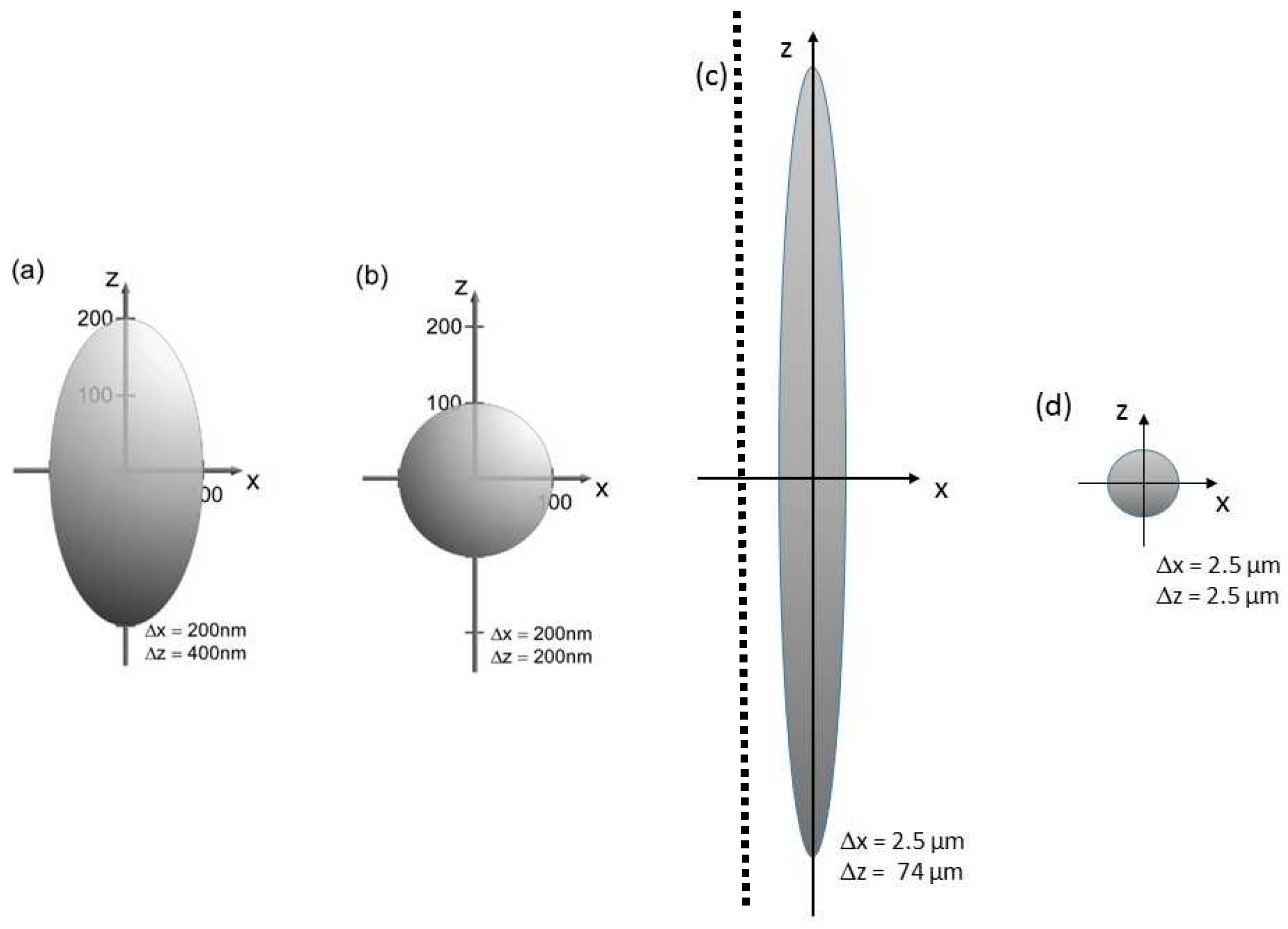
Live cell microscopy turned out to be a key discipline of biomedical sciences. Present trends of modern light microscopy include 3D applications, super-resolution microscopy, as well as low light exposure for live cell imaging. However, super-resolution methods are often restricted to single planes. They include Single Molecule Localization Microscopy (SMLM) [1,2,3,4,5,6,7,8,9,10,11,12,13,14] based on the precise localization of optically isolated single molecules in a large number of image frames. From the joint mapping of all localizations, an image with enhanced resolution is constructed. Typically, this approach is used for measuring thin layers, e.g., cell membranes, with nanometer precision, but is also being increasingly applied to thicker specimens in the micrometer range, e.g., cell nuclei [12]. Usually, comparably long acquisition times and high light exposures are required, which risk damage to living specimens, e.g., cells (see Section 4). Stimulated Emission Depletion (STED) Microscopy [15,16,17], where fluorescence from the outer region of an exciting laser spot is suppressed due to stimulated emission within the field of a second (donut) laser beam, also requires very high light exposure, whereas MINFLUX, a technique permitting single molecule tracking in the center of a donut laser spot [18,19] at enhanced localization precision, still has to prove its ability to enable super-resolution 3D imaging at sufficiently low light exposition. Patterned Illumination Microscopy methods, like Structured Illumination Microscopy (SIM) [20,21,22,23,24,25] and Spatially Modulated Illumination (SMI) Microscopy [26,27,28,29,30], permit low light doses, similar to conventional wide-field microscopy, but the enhancement of optical resolution around a factor of 2 compared to the Abbe criterion is rather modest. For optically isolated small objects, the size resolution (smallest extension to be measured) of SMI is better and may be as good as 1/15th of the exciting wavelength; however, the structure of illumination, resulting, e.g., from an optical grid, an interferometer arrangement, or a spatial light modulator, is often lost in deeper layers of a cell or tissue sample. Therefore, another approach is needed to apply established methods of 3D microscopy, e.g., Confocal Laser Scanning Microscopy (CLSM) [31,32] or Light Sheet Fluorescence Microscopy (LSFM) [33,34,35], and to replace the anisotropic optical resolution (represented by the point spread function; see Figure 1) by an isotropic resolution. As shown in Figure 1, the lateral (object plane) resolution in microscopy is generally by a factor ≥ 2 better than axial resolution, but rotation of the samples by axial tomography allows us to use the optimal resolution for each direction. This advantage becomes most distinct at lower numerical aperture AN, when the ratio between axial resolution (estimated as Δz = n λex/AN2) and lateral resolution (Δx~0.5 λex/AN) [36,37] increases inversely with the numerical aperture. For example, at AN = 1.4 (n = 1.515), this ratio is 2.2, but it increases by a factor of around 30 at AN = 0.1. In this latter case, rotation of the sample would allow an effective isotropic 3D resolution of about 2.5 µm instead of a lateral resolution of 2.5 µm together with an axial resolution of 74 µm (λex = 488 nm; n = 1.515). The 3D observation volume would be diminished by a factor of (2.5 × 2.5 × 74 µm3)/(2.5 µm)3 = 30. This number may be compared with the reduction in observation volume by a factor of (0.2 × 0.2 × 0.6 µm3)/(0.2 × 0.2 × 0.1 µm3) = 6, as achieved by 4Pi microscopy, the first experimental super-resolution method reported in [38,39,40].
However, application of axial tomography has various experimental requirements, in particular:
- -
- embedding of the cells in an appropriate medium within rotatable devices as well as precise adjustment of various angles under the microscope [41];
- -
2. Angular Resolution
Angular resolution has been used in many fields of microscopy. The oldest application may be dark field microscopy (first published in 1921 [46]), where light incidence on a sample occurs under a certain angle of inclination, so that specular reflection is avoided in the detection path. Light scattering microscopy with angular resolution has been applied to study cell morphology as well as metabolic changes, e.g., upon apoptosis or necrosis, under simultaneous visual control [47,48,49]. Detection of infiltrating tumor cells within host tissue emphasizes the potential of this method in view of label-free optical diagnostics [49].
Angular resolution plays a major role in Total Internal Reflection Fluorescence Microscopy (TIRFM) [50,51]. Using an angle of light incidence Θ above the critical angle of total internal reflection, an evanescent electromagnetic field is created, which permits selective measurements of a cell–substrate interface, e.g., cell membrane. So far, TIRFM has been applied for detection of focal adhesions, cell–substrate contacts [52], protein dynamics [53], as well as endocytosis or exocytosis [54,55]. Furthermore, variation of Θ permits modelling of cell–substrate topology with an axial resolution in the nanometer range [56]. This method has been applied successfully to distinguish cells of different malignancy or to measure the efficacy of chemotherapeutic or phototherapeutic drugs. Supercritical angles were used for excitation as well as for detection of fluorescence from thin layers [57,58], and simultaneous detection after subcritical and supercritical angle excitation allowed signals arising from inside bulk samples as well as from their surfaces to be distinguished [59].
3. Axial Tomography in 3D Microscopy
3.1. Overview
Computerized axial tomography methods to obtain 3D structural information by imaging an object from various angles using ionizing radiation have been well-established in many fields of application, from medicine to the geosciences [60,61]. Attempts to use large angle rotation of fluorescent objects located inside thin glass capillaries (or on glass fibers) to ameliorate their 3D resolution by high numerical aperture microscopy date back to the 1990s [45,62]. In these first implementations (rotation angle up to 2π) constructed for a Zeiss Axiomat Microscope (objective lens: planapochromat 100×/1.3 oil immersion), the tilting device consisted of an exchangeable quartz glass capillary, in which the biological specimen in suspension was sucked in. Typically, the capillary had an average diameter of 0.2 mm and a length of 70–80 mm, with the axis in the direction of the object plane. One end of the capillary was fixed in a bearing which itself was mounted directly into a brass block mounted into an aluminum block. The middle part of the capillary/fiber (i.e., the region of observation) was located in a long V-shaped groove of a plastic inlay. This prevented undefined lateral shifts of the capillary during rotation. Instead of the plastic inlay, it was possible to adapt an appropriate piece of glass without a groove, to implement a transmission light microscopy mode. The bearing (including the capillary) could be tilted easily with a flexible shaft by a multiprocessor-controlled stepping motor with a reproducible angular resolution of 0.2°. For the connection of the stepping motor to the bearing, a flexible shaft was used to minimize the vibrations caused by the motor to the capillary. The effective detection length in the capillary was 18.2 mm. The capillary could be moved about 2.7 mm along the object plane. With the tilting device adapted to the microscope, fluorescence, transmission, and reflection modes were possible. Instead of a capillary, it was also possible to use a glass fiber with similar or smaller diameters onto which the specimens (e.g., cells) were attached. In order to adapt the device to confocal scanning microscopes, all components were constructed of low-weight materials (typical total weight of such a tilting device: 13.6 g). To improve imaging quality, a cover glass can be inserted between the objective lens and the capillary/fiber, still facilitating the possibility to focus through the entire capillary/fiber. In order to minimize image distortion caused by the capillary/glass fiber, the refractive index of the mounting medium was matched to that of the quartz glass capillary (or glass fiber) used. This was achieved in the case of the capillary by using a glycerol–water mixture as the buffer medium for the specimens as well as the mounting medium around the capillary. For the use of a glass fiber, the refraction index of the mounting medium was matched to the glass type of the fiber; if a special mounting medium had to be applied for biological reasons, an appropriate glass type with an adequate refractive index can be chosen.
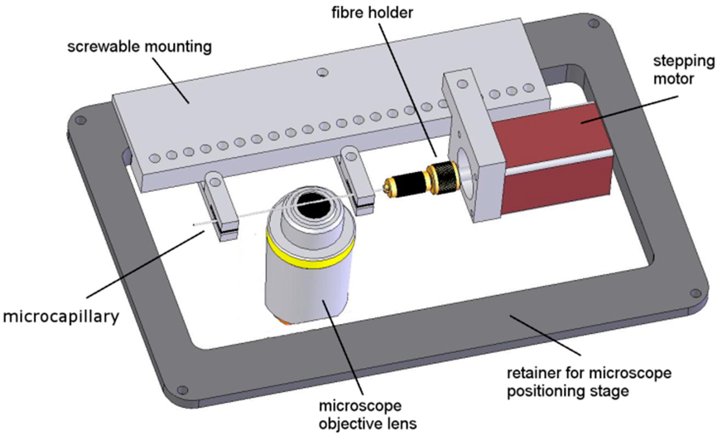
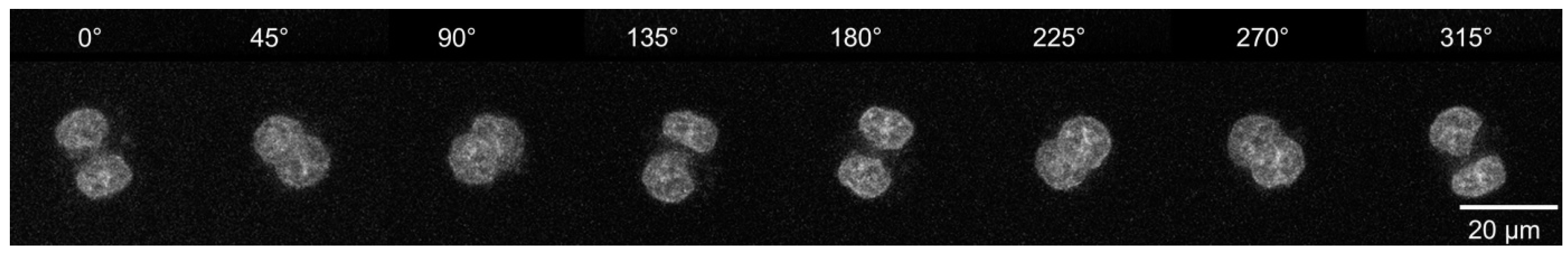
With such devices, 3D distance measurements with a precision of a few tens of nanometers were achieved. Using localization microscopy with appropriate differences in the spectral signature, this would correspond to an optical 3D resolution in the nanometer range. Further improvement of axial tomography in 3D microscopy was realized in the early 2000s, when Heintzmann and Cremer [42] as well as Matula et al. [63] described that tilting or rotation of a sample in combination with multi-view microscopy improved the 3D resolution considerably. In 2009, an optical projection tomography microscope generating 3D images of single cells with isometric high resolution in absorption and fluorescence mode was described [64]. Cells were suspended in an optical gel flow through a custom-designed micro-capillary, and multiple projection images were taken by rotating the micro-capillary. After alignment of these projection images, computed tomography methods were applied to create a 3D reconstruction, which enabled spatial resolution of fluorescence around 350 nm in both axial and lateral dimensions. Test particles were fixed on glass fibers, optically localized with high precision, and automatically rotated to obtain views from different perspective angles. From various angular views, 3D distances were calculated with a precision in the ten nanometer range. As a proof of concept, the spindle apparatus of a mouse oocyte during the metaphase II stage was imaged [65]. Further experiments of living cells, however, would need some different equipment. An experimental setup, where single cells are grown in a cultivation medium, located within micro-capillaries and observed from different sides after adaptation of an innovative sample holder to the x,y-stage of an inverted microscope, is reported in [41,66] (Figure 2). The cultivation medium may be liquid (e.g., in combination with microfluidics [41]) or solid (e.g., agarose), where the latter case is particularly interesting for single-cell experiments [66]. To minimize optical aberrations in an air environment (using a 10–20× magnifying objective lens), rotatable cylindrical glass capillaries of 550 µm outer diameter were inserted and optically coupled (by an immersion fluid) to rectangular glass capillaries of 600 µm × 600 µm inner cross-section. Hence, light in confocal as well as in light sheet microscopy was always incident on the rectangular surfaces. At high magnification with a water immersion objective lens (63×/0.90), cylindrical FEP (fluoroethylene propylene) [67] capillaries were used whose refractive index of 1.33–1.35 fitted those of the sample as well as the water immersion and ensured optimum imaging independent of the sample geometry. In this case, no second (outer) capillary was needed. For rotation of the inner glass or the FEP capillary by arbitrary angles up to 360°, the capillary was coupled by a specific fiber holder to a computerized stepping motor with micro-step positioning control and an angular resolution of 0.45°, and z-stacks were recorded for various angles using confocal or light sheet microscopy. Use of single or dual micro-capillaries did not have any influence on resolution and stability of the whole system. Three-dimensional images or z-projections were calculated for each angle, as depicted in Figure 3 at steps of 45° for two adjacent HeLA cervical carcinoma cells incubated for 2 h with the fluorescent cytotoxic agent doxorubicin [66]. Doxorubicin accumulates in the cell nuclei, which, depending on the angle of detection, appear either superimposed or separate. Reduction in the information obtained under variable angles to one image with isotropic resolution requires some specific software, e.g., a method of maximum likelihood [68], which only recently could be adapted to the results of [66] (E. Herzog et al., Focus on Microscopy, Porto, source code: https://github.com/viol4nce/AxialTomo-Registration-and-Visualisation-Suite, accessed on 2–5 April 2023).
3.2. 3D Distance Measurements at the Nanoscale
In a variety of applications, precise 3D distance measurements between fluorescence labeled targets are required. Biomedical examples of this are the correct determination of 3D distances between breakpoint regions in human cells. Such distances may influence the probability of radiation-induced oncogenic translocations. Another application example would be measurements of the 3D distance of specific DNA sequences with respect to the center of a specific compact gene domain in the cell nucleus. For the initiation of transcription and hence gene regulation, it may be essential, whether a DNA target sequence is located at the periphery of a compact domain, or inside such a domain. In the latter case, the probability of transcription initiation may strongly depend on the distance of such a target sequence from a compact domain surface [69,70,71,72]. Axial tomography permits a substantial improvement of the precision of 3D distance measurements using a conventional confocal microscopy device [31].
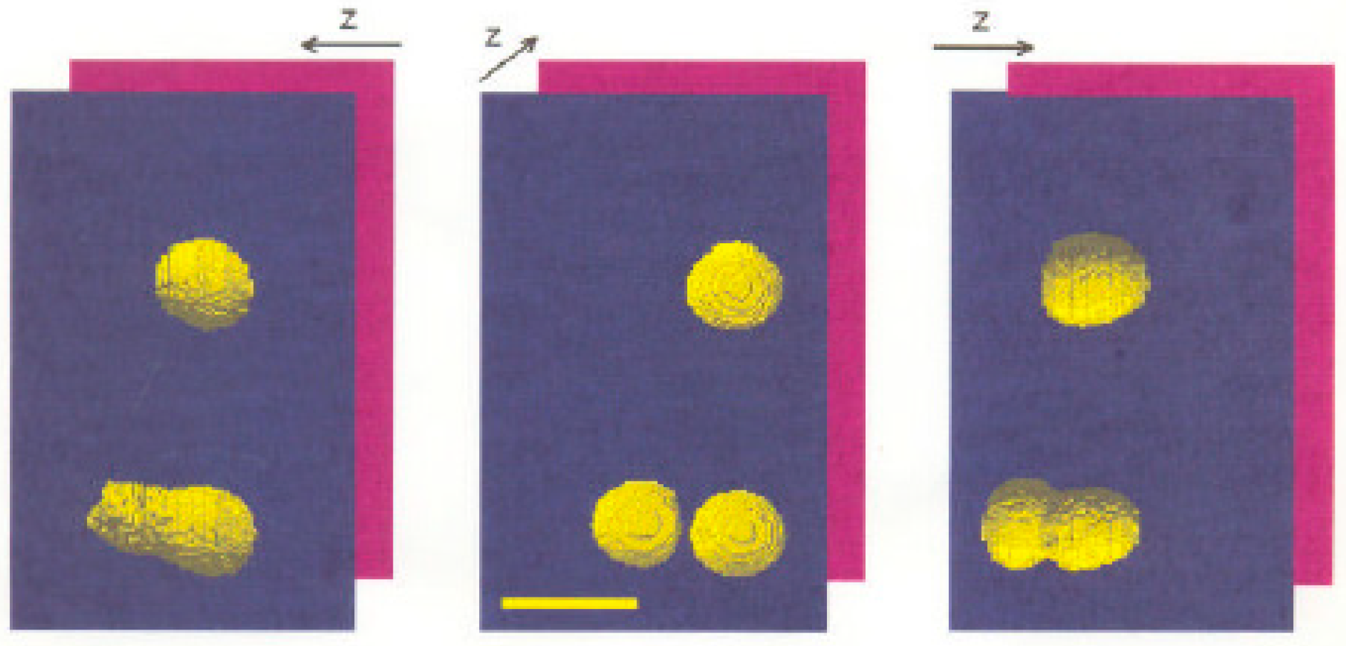
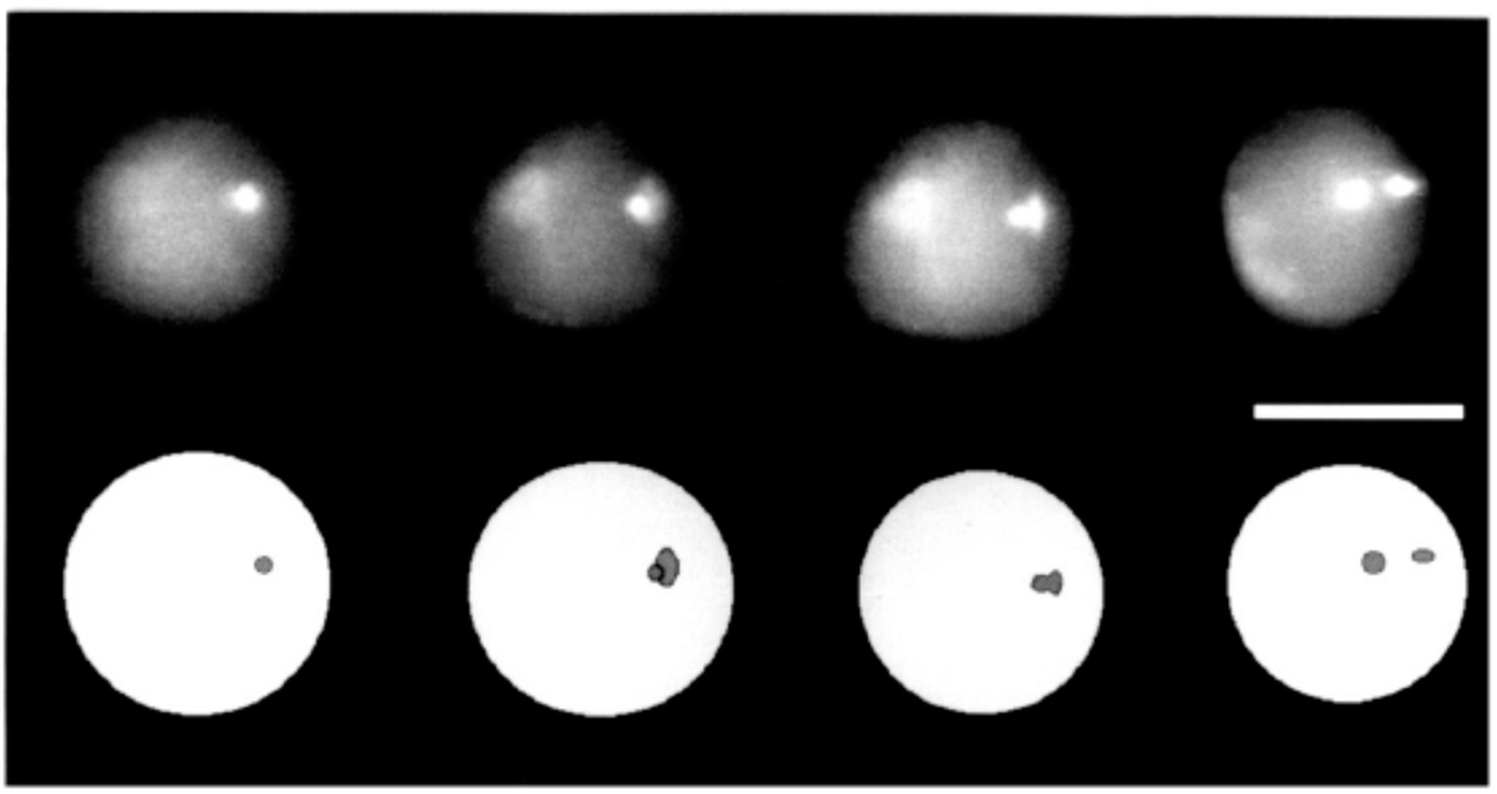
In a “proof-of-principle” experiment, a versatile tilting device based on [62] was applied. It consisted of an exchangeable quartz glass capillary with an average diameter of 0.2 mm and a length of 70–80 mm, in which the specimen in suspension can be sucked in. The axis of object rotation was perpendicular to the optical axis of the microscope. For fluorescence registration, an AN = 1.4 objective lens was used (for further details, see above). Figure 4 shows an example of fluorescent calibration beads imaged from different directions. “Optically fused” objects could be identified as single separated objects after rotation into the optimal perspective, where they were located in the same focal plane. By choosing the right perspective, it was also possible to determine the shape of all targets correctly.
To summarize, axial tomography in combination with standard microscopy devices allows us to determine (within the limits of the object plane resolution used) the 3D shape of objects correctly. Furthermore, it enables quantitative high-precision 3D measurements. Since localization precision is dependent on the half width of the point spread function [12], axial tomography might advantageously be used to also enhance the 3D resolution in Single Molecule Localization Microscopy (SMLM), by rotating the molecules into an appropriate perspective. This should be especially interesting, if low numerical aperture objective lenses are used for extremely large working distances [73] or fields of view. For example, by use of an objective lens of AN = 0.28 for a very large field of ~1 cm2 [74] to study the nuclear chromatin nanostructure of cells by SMLM in a large tissue section, the localization precision along the optical axis would be reduced by a factor of n/(0.5 AN) = 9.3 (λex = 488 nm, n = 1.3). If a localization precision in the (x,y) object plane of σxy~20 nm is assumed, the axial precision would be σz~9 × 20 nm = 180 nm only, and the corresponding optical resolution 2.35 σz~420 nm [12]. For many distance measurements (e.g., the position of target sequences in nuclear gene domains; see above), this would not be sufficient.
To enhance under these low numerical aperture conditions the localization precision to 20 nm along the optical axis as well, one would need to register 9 × 9 more fluorescence photons (e.g., 400,000 photons/molecule instead of 5000/molecules [13], which would be difficult to achieve in typical SMLM applications), or at least substantially slow down the SMLM imaging process to obtain a highly enhanced resolution [14]. Another solution might be to enhance the axial localization precision by appropriately designed structured illumination methods [30]. By choosing the right axial tomographic perspective, however, the precision of 3D position/distance measurements may be enhanced several times even using state-of-the-art low numeric aperture microscopy with large working distances.
3.3. Axial Tomography to Study the 3D Distribution of Selected Chromatin Sites
The three-dimensional distribution of chromatin in the cell nucleus has been a topic of extensive research [75,76,77]. The more the 3D resolution and the precision of 3D distance measurements are enhanced, the more structural information may be obtained [78,79]. As an example of the application of axial tomography in chromatin structure analysis, the position of peri- or paracentromeric chromosomal targets was examined [80]. Nuclei with specifically stained chromosome targets were placed in a glass capillary, similar to the scheme shown in Figure 2. This design made it possible to choose an x, y-plane for any two object points (e.g., gravity centers of two hybridization signals), where both object points are in focus. Accordingly, the much better lateral resolution of the light microscope was exploited to achieve a true 3D distance measurement between the two points of interest.
For a comparison of the 3D distribution of target regions from different chromosome territories [78] in the same population of cell nuclei, two color fluorescence in situ hybridization (FISH) experiments were carried out with probes delineating either the chromosomal domains 1q12 and 15p1 or 7c and 17c. To avoid problems which might have possibly resulted from chromatic aberrations when two target regions were stained with different fluorochromes, labeling of all targets in one nucleus was performed with one fluorochrome for axial tomographic measurements, while a second fluorochrome was used to achieve a discrimination between heterologous targets. An example of a human lymphocyte is given in Figure 5.
3.4. Computational Reconstruction of 3D Images from Axial Tomography Data
Axial tomography allows us to obtain a series of microscopy images of a 3D specimen viewed from different angles. Like in confocal or in structured illumination microscopy, where series of images from the same object differing in one defined aspect are used to reconstruct 3D images, axial tomographic images may be computationally combined to obtain 3D images with an enhanced isotropic resolution comparable to the lateral resolution of a single deconvoluted dataset. Axial tomographic imaging in combination with simultaneous data reconstruction also opens the possibility for a more precise quantification of 3D data. In an approach developed by Heintzmann et al. [42,81], the algorithm automatically determines the relative angles of rotation, aligns the data from different rotational views, and reconstructs a single high-resolution 3D dataset. The reconstruction makes use of a known point spread function and is based on an unconstrained maximum likelihood (ML) deconvolution. Iterative ML reconstruction is a widely used tool for deconvolution of confocal data. This technique has been further extended to include the data of the specimen imaged under different rotational views in the process of ML reconstruction (see also Supplementary Material).
The reconstruction algorithm was applied to simulated as well as to experimental confocal datasets. The gain in resolution was quantified, and the effect of choice of adaptive parameters on the speed of convergence was investigated. A clearly improved 3D resolution was obtained by axial tomography together with reconstruction as compared with reconstruction of confocal data from only a single angular view (Figure 6).
3.5. Application of Axial Tomography in Embryology
Instead of a micro-capillary, the object may also be fixed to a special glass fiber, which is then rotated in the object space of the microscope lens. A stepwise fiber rotation can be controlled by a miniaturized stepping motor incorporated into the device. As an application in embryology [65], the spindle apparatus of a mature mouse oocyte was imaged during metaphase II meiotic arrest under different perspectives (Figure 7). Very few images only registered under different rotation angles were sufficient for full 3D reconstruction. This may be compared to 3D SIM generated images, where several dozens of images are required for a full 3D reconstruction. Although such 3D SIM images allow a superior 3D resolution, they also enhance the photon load and the risk of bleaching.
3.6. Combination of Axial Tomography and Structured Illumination (SIM)
The 3D resolution may be further enhanced by the combination of Structured Illumination Microscopy (SIM) with axial tomography [82]. An example is given in Figure 8 for autofluorescence measurements of a leaf of Cedrus deodora (Himalayan cedar). In such a combination of SIM with axial tomography, the contrast is enhanced, and a resolution around 2 µm is attained, even at the rather low numerical aperture of AN = 0.25.
3.7. Axial Tomography of Very Large Transparent Objects: Combination with Ring-Array Microscopy
To study very large transparent objects like embryos in a more advanced stage, cleared tissue volumes (i.e., of sufficient transparency and homogeneity [83]) in cancer research, or cleared brain in neurobiology, light sheet microscopy (LSM) methods have been most successfully applied [33]. In these approaches, a thin light sheet (a few µm waist thickness) is used to illuminate various sections of the object. At each section, an image is taken perpendicular to the light sheet plane, and a 3D image is computed. If, for example, the light sheet method would be applied to a transparent structure of 1 cm thickness, the numerical aperture of the objective lens should be around 0.4 when using an excitation wavelength of 488 nm and a refraction index of 1.3 (water). Without the light sheet, this would result in a limiting optical resolution of about 600 nm laterally and 4 µm axially, with an observation volume of [4/3π × 0.6/2 × 0.6/2 × 4/2] µm3 = 0.75 µm3. By axial tomographic rotation, e.g., of an embryo, the effective 3D observation volume would be reduced to [4/3π × 0.6/2 × 0.6/2 × 0.6/2] µm3 = 0.11 µm3, i.e., the effective 3D resolution would be enhanced by a factor of 7. At all angles, however, the entire object volume would be fully illuminated. Using, in addition, a light sheet with 5 µm waist diameter for studying large objects, the illuminated object volume may be substantially reduced, thus minimizing adverse effects of phototoxicity and photobleaching.
A still more radical enhancement of axial tomographic 3D resolution of very large and thick transparent objects might be obtained by an imaging system with a substantially larger numerical aperture than, e.g., 0.4, as in the previous example, while maintaining the large working distance (e.g., 1 cm, or even larger). This might be achieved by a novel fluorescence microscopy concept [73]; such “Ring-Array Microscopy” approaches should enable a direct integration of Super-Resolution Microscopy (SRM) methods (SIM/Nanosizing, STED, SMLM, MINFLUX, SIMFLUX) into low aperture microscopy systems with working distances up to the multi-centimeter range and fields of view (FOVs) up to ≥1 cm2, while still permitting nanometer-scale resolution. To achieve this goal, a “synthetic aperture” coherent illumination mode is created with multiple, constructively interfering excitation beams positioned in a “Ring-Array“ arrangement around a beam-free interior zone containing low aperture instrumentation for fluorescence collection. A combination of Ring-Array Microscopy, axial tomography, and Light Sheet microscopy is envisaged to eventually permit studies of selected sites in intact, very thick transparent specimens (e.g., 1 cm or more in diameter) with a resolution approaching the nanometer scale [30].
An application example of Ring-Array Microscopy might be the analysis of nuclear genome structure in selected nuclei in large tissues to study, e.g., the heterogeneity of cancer-related nuclear structure [84]. Since chromatin nanostructure is intimately connected with essential cellular functions like transcription, replication, and repair [69,70,71,72,85], the analysis of such chromatin nanostructures of cells in their environment (e.g., a tissue) is of great importance. Another potential field of application is enhanced 3D resolution analysis of nuclear chromatin structure of neurons in intact cleared brain tissue, supposed to be correlated with long-term memory [86]. Since many of the chromatin structures involved have typical sizes in the 100 nm range, one would need an appropriately enhanced resolution; such a resolution might be provided even at the extreme distances required for the analysis of large brain sections by combination with Ring-Array microscopy.
4. Discussion
For many biomedical applications, methods are essential to enhance the three-dimensional (3D) resolution of an optical microscope. Axial tomography (AT) permits the rotation of the microscopic object into the best perspective required for optimal imaging, making possible a 3D resolution corresponding to the best resolution of the system (usually that of the object plane). Here we present some applications of this technique to improve nuclear genome structure analysis, to image the spindle apparatus in a single mouse oocyte, to study the effects of a cytotoxic agent on single cells, to combine axial tomography and Structured Illumination Microscopy (SIM) for enhancement of the resolution of autofluorescent structures in a single cell of Cedrus deodora (using a low numerical aperture objective lens), or to reconstruct computationally the three-dimensional shape of a multi-cellular aggregate.
During recent decades, laser-assisted light microscopy at enhanced resolution has made very substantial progress, presently approaching an optical resolution down to the Angström range [14,29]. Nonetheless, even in this context, axial tomography still provides a variety of interesting features.
4.1. Simplicity
Axial tomography is a technically relatively simple device which allows us to position a three-dimensional object in such a way that the microscopic observation is optimized. For this, any microscopic procedure may be applied, from simple magnifying lenses to highly sophisticated super-resolving MINFLUX systems. Since the object plane resolution is commonly better than the axial resolution, two closely adjacent object sites can be resolved and their 3D distance correctly measured just by rotating the object in such a way that the two sites are located in the object plane. For this, even visual observation alone would already be sufficient to provide an enhanced optical 3D resolution corresponding to that achieved without axial tomography. If the image is registered by an appropriate CCD or sCMOS sensor, a 3D image may be computed with an enhanced isotropic optical resolution from the image frames taken at various rotation angles. For example, in combination with a smartphone-based device [87], the combination of axial tomography and computational reconstruction is envisaged to allow a 3D resolution down to the nanometer range. Due to the comparatively low costs of such a setup, this should allow parallel studies not exceeding the instrumental costs of a present commercial high-resolution microscopy device.
It should be emphasized that axial tomography is not a competitive method to any existing 3D method, e.g., confocal or light sheet microscopy, but may be used in combination with those methods, whose lateral resolution is maintained, while an isotropic resolution is generated. Use of axial tomography requires a larger number of light exposures and thus a higher photon budget. If, for example, z-stacks of 30 images (recorded by confocal or light sheet microscopy) are measured at eight angles, a total number of 240 images are needed for one object. This means that in the case of confocal laser scanning microscopy, the whole sample is exposed to light 240 times, whereas for light sheet microscopy, each “plane” is illuminated 8 times. In previous studies [88], we reported that non-phototoxic light doses applied to native cells range between 25 and 200 J/cm2 (depending on the wavelength of illumination) and are around 10 J/cm2 when using fluorescent dyes or fluorescent proteins. Assuming low light exposure around 100 mW/cm2 (similar to solar irradiance) and an illumination time of 1 s per image, about 100 images can be recorded in the latter case under non-phototoxic conditions. Therefore, with respect to cell viability, axial tomography can be effectively combined with light sheet microscopy, but should be regarded with care when using confocal microscopy methods. It should be mentioned that neither the signal-to-noise ratio (SNR) nor the field of view (FOV) change due to this combination of methods.
Axial tomography needs mechanical adjustment of all angles, and even with a stable and fully computerized setup, as depicted in Figure 2, one would need a minimum of 2 s for recording images at eight angles by wide-field microscopy. When applying depth-resolving techniques (again with mechanical adjustment of a light sheet or a confocal plane), this time, they should be multiplied by a factor of around 30, and some additional time for offline evaluation should be added. Therefore, the method of axial tomography presently does not seem to be appropriate for dynamic imaging at short time scales. However, multiple measurements with intervals of some minutes up to hours appear clearly possible, as reported below.
4.2. Multiple Measurements of the Same Object
Axial tomography allows us to obtain multiple images of the same object from a variety of defined rotation angles. This enables us to measure image features much more accurately. For example, an essential problem in multi-color super-resolution 3D microscopy is the precise determination of the chromatic shift at different axial positions of the fluorophore. The transcriptional activity of a gene may critically depend on the position of transcription factor binding sites within a gene domain [69,70,71,72,85]. For this, it may be required to measure 3D distances down to the nanometer range between sites labelled with different spectral signatures. Therefore, the chromatic shift also has to be calibrated with an error in the nanometer range. This becomes possible by axial tomographic measurement of the chromatic shift at different rotation angles (and hence axial positions).
4.3. Deep View Imaging of Very Large Objects
A major challenge to realizing a sufficient 3D resolution of extended objects like thick tissue sections, embryos, organoids, or spheroids is the large working distance required for enhanced 3D resolution. For example, for a transparent thick object requiring the use of an objective lens with a numerical aperture of AN = 0.1, the optical resolution would be about 2.5 µm in the object plane, but about 75 µm along the optical axis. In this case, axial tomography would permit us to enhance the optical 3D resolution of the numerically reconstructed image volume by a factor of 30. In combination with other approaches like Ring-Array microscopy [73], the implementation of super-resolution approaches should be feasible, thus enabling a 3D super-resolution even of intact thick transparent objects, e.g., organisms studied in developmental biology, cancer specimens, brain samples, or organoids.
For example, recent super-resolution microscopy (SRM) analyses [29,74] indicated that the density of small compact domains should be sufficiently high to restrict the accessibility and hence the binding of transcription factor complexes (TFCs) to target sequences within such small domains [69]. As a consequence, the initiation of transcription depends not only on the folding pattern of the chromatin fiber (as obtained, e.g., by biochemical approaches) but also on the local absolute DNA density (Mbp/µm3), i.e., on the ratio between the DNA content (bp) divided by the volume occupied. For a correct domain volume (Vdomain) determination, however, a 3D observation volume Vobs ≤ Vdomain is required. While with high AN-based SRM, a 3D observation volume equivalent to a spherical domain diameter down to ~40 nm has been achieved [70], Vobs increases substantially with smaller AN (see above). Using AT-based deep view imaging, it should become possible to elucidate the heterogeneity of chromatin density-related control of transcription in nuclei, even in thick transparent tissue specimens, down to domain diameters in the ~100 nm range.
4.4. Molecular Imaging/FRET
Information on intra- or intermolecular interactions can be obtained by introducing spectral or temporal (e.g., fluorescence lifetime) information. A prominent example is Förster Resonance Energy Transfer (FRET) from an excited donor molecule to an acceptor molecule which is able to fluoresce [89]. Since this interaction is limited to distances below 10 nm, molecular interactions in the nanometer range may be evaluated upon application of pharmacological agents as well as in various scenarios of disease or cell death (for reviews, see [90,91,92,93,94]). Experimental parameters are either the intensity ratio of acceptor and donor fluorescence determined from the emission spectra, or the fluorescence lifetime of the donor, which is shortened in the case of energy transfer. Axial tomography may help to identify the cellular sites of molecular interaction at enhanced 3D resolution, but without the need for nanometer image resolution.
Fluorescence lifetime imaging (FLIM) is a well-established technique based either on wide-field or on laser scanning microscopy (LSM). In the first case, ultra-fast (picosecond) [95,96,97] or phase-resolving camera systems [98,99,100,101,102,103] are used, whereas in the second case, LSM with additional time sensitivity is [104,105,106,107] applied. Measuring times may be quite short (2–10 s) in the first case, but rather long (≥30 s) in the second case. Taking into account that for 3D microscopy, several planes should be recorded and that for axial tomography, various angles are needed, the total light exposure is considerably higher than for steady-state microscopy, thus often exceeding the limit of non-phototoxic light doses. Phototoxicity, however, may be avoided when combining camera-based wide-field microscopy (e.g., light sheet microscopy [96,103]) with axial tomography.
4.5. Final Remarks Concerning 3D Reconstruction
For image reconstruction from various angular views, methods of maximum likelihood were applied using either gradient-based [108] or Fourier transform [42] techniques. Due to their generally eccentric location within micro-capillaries, cells recorded at various angles not only had to be rotated by software to their original position, but also shifted for an optimum overlay in order to obtain information from all individual images. An alternative method is based on fluorescent markers used as supporting points [67], which, however, need to be clearly identified in all images. This method only works if cells can be stained with appropriate fluorescent beads, and if the fluorescent background is not too strong. It could not be applied for the examples given here. Three-dimensional reconstruction algorithms may be combined with further modern imaging or deep learning algorithms. A description of these techniques, however, would exceed the scope of the present hardware-based manuscript.
Supplementary Materials
The following supporting information can be downloaded at https://www.mdpi.com/article/10.3390/biophysica4020010/s1. Reference [81] is cited in the supplementary materials.
Author Contributions
H.S. and C.C. contributed equally to all parts from conceptualization up to writing of this manuscript. All authors have read and agreed to the published version of the manuscript.
Funding
This research received no external funding.
Institutional Review Board Statement
Not applicable.
Informed Consent Statement
Not applicable.
Data Availability Statement
Not applicable.
Acknowledgments
For the development of the axial tomographic method reviewed in this manuscript, we thank our collaborators and colleagues, especially Harald Bornfleth, Joachim Bradl, Sarah Bruns, Thomas Bruns, Thomas Cremer, Steffen Dietzel, Heinz Eipel, Markus Durm, Peter Edelmann, Volker Ehemann, Roland Eils, Arif Esa, Alexei V. Evsikov, Michael Hausmann, Rainer Heintzmann, Elias Herzog, Tobias Aurelius Knoch, Michael Kozubek, Gregor Kreth, Petr Matulla, Christian Münkel, Verena Richter, Bernhard Rinke, Bernhard Schneider, Florian Staier, Michael Wagner, Eva Weilandt, Florian Schock, and Ernst H. K. Stelzer.
Conflicts of Interest
The authors declare no conflicts of interest.
References
- Betzig, E. Proposed method for molecular optical imaging. Opt. Lett. 1995, 20, 237–239. [Google Scholar] [CrossRef]
- Hess, S.; Girirajan, T.; Mason, M.D. Ultra-High Resolution Imaging by Fluorescence Photoactivation Localization Microscopy. Biophys. J. 2006, 91, 4258–4272. [Google Scholar] [CrossRef] [PubMed]
- Bock, H.; Geisler, C.; Wurm, C.A.; von Middendorff, C.; Jakobs, S.; Schoenle, A.; Egner, A.; Hell, S.W.; Eggeling, C. Two-color far-field fluorescence nanoscopy based on photoswitchable emitters. Appl. Phys. B 2007, 88, 161–165. [Google Scholar] [CrossRef]
- Huang, B.; Wang, W.; Bates, M.; Zhuang, X. Three-dimensional super-resolution imaging by stochastic optical reconstruction microscopy. Science 2008, 319, 810–813. [Google Scholar] [CrossRef] [PubMed]
- Heilemann, M.; van de Linde, S.; Schüttpelz, M.; Kasper, R.; Seefeldt, B.; Mukherjee, A.; Tinnefeld, P.; Sauer, M. Sub-diffraction-resolution fluorescence imaging with conventional fluorescent probes. Angew. Chem. Int. Ed. Engl. 2008, 47, 6172–6176. [Google Scholar] [CrossRef] [PubMed]
- Biteen, J.S.; Thompson, M.A.; Tselentis, N.K.; Bowman, G.R.; Shapiro, L.; Moerner, W.E. Single-molecule active-control microscopy (SMACM) with photo-reactivable EYFP for imaging biophysical processes in live cells. Nat. Methods 2008, 5, 947–949. [Google Scholar] [CrossRef]
- Betzig, E.; Patterson, G.H.; Sougrat, R.; Lindwasser, O.W.; Olenych, S.; Bonifacino, J.S.; Davidson, M.W.; Lippincott-Schwartz, J.; Hess, H.F. Imaging Intracellular Fluorescent Proteins at Nanometer Resolution. Science 2006, 313, 1642–1645. [Google Scholar] [CrossRef] [PubMed]
- Rust, M.J.; Bates, M.; Zhuang, X. Sub-diffraction-limit imaging by stochastic optical reconstruction microscopy (STORM). Nat. Methods 2006, 3, 793–796. [Google Scholar] [CrossRef]
- Cox, S.; Rosten, E.; Monypenny, J.; Jovanovic-Talisman, T.; Burnette, D.T.; Lippincott-Schwartz, J.; E Jones, G.; Heintzmann, R. Bayesian localization microscopy reveals nanoscale podosome dynamics. Nat. Methods 2011, 9, 195–200. [Google Scholar] [CrossRef]
- Lidke, K.A.; Rieger, B.; Jovin, T.M.; Heintzmann, R. Super-resolution by localization of quantum dots using blinking statistics. Opt. Express 2005, 13, 7052–7062. [Google Scholar] [CrossRef]
- Cremer, C.; Masters, B.R. Resolution enhancement techniques in microscopy. Eur. Phys. J. 2013, 38, 281–344. [Google Scholar] [CrossRef]
- Cremer, C.; Szczurek, A.; Schock, F.; Gourram, A.; Birk, U. Super-resolution microscopy approaches to nuclear nanostructure imaging. Methods 2017, 123, 11–32. [Google Scholar] [CrossRef] [PubMed]
- Lelek, M.; Gyparaki, M.T.; Beliu, G.; Schueder, F.; Griffie’, J.; Manley, S.; Jungmann, R.; Sauer, M.; Lakadamyali, M.; Zimmer, C. Single-molecule localization microscopy. Nat. Rev. Methods Primers 2021, 1, 39. [Google Scholar] [CrossRef] [PubMed]
- Reinhardt, S.C.M.; Masullo, L.A.; Baudrexel, I.; Steen, P.R.; Kowalewski, R.; Eklund, A.S.; Strauss, S.; Unterauer, E.M.; Schlichthaerle, T.; Strauss, M.T.; et al. Ångström-resolution fluorescence microscopy. Nature 2023, 617, 711–716. [Google Scholar] [CrossRef] [PubMed]
- Hell, S.W.; Wichmann, J. Breaking the diffraction resolution limit by stimulated emission: Stimulated-emission-depletion fluorescence microscopy. Opt. Lett. 1994, 19, 780–782. [Google Scholar] [CrossRef]
- Wildanger, D.; Medda, R.; Kastrup, L.; Hell, S. A compact STED microscope providing 3D nanoscale resolution. J. Microsc. 2009, 236, 35–43. [Google Scholar] [CrossRef] [PubMed]
- Hell, S.W. Far-Field Optical Nanoscopy. Science 2007, 316, 1153–1158. [Google Scholar] [CrossRef]
- Balzarotti, F.; Eilers, Y.; Gwosch, K.C.; Gynnå, A.H.; Westphal, V.; Stefani, F.D.; Elf, J.; Hell, S.W. Nanometer resolution imaging and tracking of fluorescent molecules with minimal photon fluxes. Science 2017, 355, 606–612. [Google Scholar] [CrossRef]
- Liu, S.; Hoess, P.; Ries, J. Super-Resolution Microscopy for Structural Cell Biology. Annu. Rev. Biophys. 2022, 51, 301–326. [Google Scholar] [CrossRef]
- Lukosz, W. Optical systems with resolving powers exceeding the classical limit, Part 1. J. Opt. Soc. Am. 1966, 56, 1463–1472. [Google Scholar] [CrossRef]
- Lukosz, W. Optical systems with resolving powers exceeding the classical limit, Part II. J. Opt. Soc. Am. 1967, 57, 932–941. [Google Scholar] [CrossRef]
- Gustafsson, M.G.L. Surpassing the Lateral Resolution Limit by a Factor of Two Using Structured Illumination Microscopy. J. Microsc. 2000, 198, 82–87. [Google Scholar] [CrossRef] [PubMed]
- Heintzmann, R.; Cremer, C. Laterally modulated excitation microscopy: Improvement of resolution by using a diffraction grating. Proc. SPIE 1999, 356, 185–196. [Google Scholar]
- Gustafsson, M.G.; Shao, L.; Carlton, P.M.; Wang, C.J.R.; Golubovskaya, I.N.; Cande, W.Z.; Agard, D.A.; Sedat, J.W. Three-Dimensional Resolution Doubling in Wide-Field Fluorescence Microscopy by Structured Illumination. Biophys. J. 2008, 94, 4957–4970. [Google Scholar] [CrossRef] [PubMed]
- Hirvonen, L.M.; Wicker, K.; Mandula, O.; Heintzmann, R. Structured illumination microscopy of a living cell. Eur. Biophys. J. 2009, 38, 807–812. [Google Scholar] [CrossRef]
- Bailey, B.; Farkas, D.; Taylor, D.L.; Lanni, F. Enhancement of axial resolution in fluorescence microscopy by standing-wave excitation. Nature 1993, 366, 44–48. [Google Scholar] [CrossRef]
- Lanni, F.; Bailey, B.; Farkas, D.; Taylor, D.L. Excitation field synthesis as a means for obtaining enhanced axial resolution in fluorescence microscopes. Bioimaging 1993, 1, 187–196. [Google Scholar] [CrossRef]
- Neil, M.A.; Juskaitis, R.; Wilson, T. Method of obtaining optical sectioning by using structured light in a conventional microscope. Opt. Lett. 1997, 22, 1905–1907. [Google Scholar] [CrossRef]
- Cremer, C.; Birk, U. Spatially modulated illumination microscopy: Application perspectives in nuclear nanostructure analysis. Philos. Trans. R. Soc. A 2022, 380, 20210152. [Google Scholar] [CrossRef]
- Birk, U. Super-Resolution Microscopy—A Practical Guide; Wiley-VCH: Weinheim, Germany, 2017; 408p, ISBN 978-3-527-34133-7. [Google Scholar]
- Pawley, J.B. Handbook of Biological Confocal Microscopy, 3rd ed.; Springer: Boston, MA, USA, 2006. [Google Scholar] [CrossRef]
- Webb, R.H. Confocal optical microscopy. Rep. Prog. Phys. 1996, 59, 427–471. [Google Scholar] [CrossRef]
- Huisken, J.; Swoger, J.; del Bene, F.; Wittbrodt, J.; Stelzer, E.H.K. Optical sectioning deep inside live embryos by SPIM. Science 2004, 305, 1007–1009. [Google Scholar] [CrossRef]
- Pampaloni, F.; Chang, B.-J.; Stelzer, E.H. Light sheet-based fluorescence microscopy (LSFM) for the quantitative imaging of cells and tissues. Cell Tissue Res. 2015, 360, 129–141. [Google Scholar] [CrossRef] [PubMed]
- Santi, P.A. Light Sheet Fluorescence Microscopy. J. Histochem. Cytochem. 2011, 59, 129–138. [Google Scholar] [CrossRef]
- Hou, W.; Wei, Y. Evaluating the resolution of conventional optical microscopes through point spread function measurement. iScience 2023, 26, 107976. [Google Scholar] [CrossRef]
- Booth, M. Adaptive Optics for Microscopy, In Microscope Resolution Estimation and Normalised Coordinates (1.0). 2020. [CrossRef]
- Hell, S.; Stelzer, E.H.K. Properties of a 4Pi confocal fluorescence microscope. J. Opt. Soc. Am. 1992, 9, 2159–2166. [Google Scholar] [CrossRef]
- Hänninen, P.E.; Hell, S.W.; Salo, J.; Soini, E.; Cremer, C. Two-photon excitation 4Pi confocal microscope: Enhanced axial resolution microscope for biological research. Appl. Phys. Lett. 1995, 66, 1698–1700. [Google Scholar] [CrossRef]
- Bahlmann, K.; Jakobs, S.; Hell, S.W. 4Pi-confocal microscopy of live cells. Ultramicroscopy 2001, 87, 155–164. [Google Scholar] [CrossRef]
- Bruns, T.; Schickinger, S.; Schneckenburger, H. Single plane illumination module and micro-capillary approach for a wide-field microscope. J. Vis. Exp. 2014, 90, e51993. [Google Scholar] [CrossRef]
- Heintzmann, R.; Cremer, C. Axial tomographic confocal fluorescence microscopy. J. Microsc. 2002, 206, 7–23. [Google Scholar] [CrossRef] [PubMed]
- Preibisch, S.; Saalfeld, S.; Schindelin, J.; Tomancak, P. Software for bead-based registration of selective plane illumination microscopy data. Nat. Methods 2010, 7, 418–419. [Google Scholar] [CrossRef]
- Landis, W.J.; Song, M.J.; Leith, A.; McEwen, L.; McEwen, B.F. Mineral and organic matrix interaction in normally calcifying tendon visualized in three dimensions by high-voltage electron microscopic tomography and graphic image reconstruction. J. Struct. Biol. 1993, 110, 39–54. [Google Scholar] [CrossRef] [PubMed]
- Bradl, J.; Hausmann, M.; Ehemann, V.; Komitowski, D.; Cremer, C. A tilting device for three-dimensional microscopy: Application to in situ imaging of interphase cell nuclei. J. Microsc. 1992, 168, 47–57. [Google Scholar] [CrossRef]
- Gage, S.H. Special oil immersion objectives for dark-field microscopy. Science 1921, 54, 567–569. [Google Scholar] [CrossRef] [PubMed]
- Cottrell, W.J.; Wilson, J.D.; Foster, T.H. Microscope enabling multimodality imaging, angle-resolved scattering, and scattering spectroscopy. Opt. Lett. 2007, 32, 2348–2350. [Google Scholar] [CrossRef] [PubMed]
- Rothe, T.; Schmitz, M.; Kienle, A. Angular and spectrally resolved investigation of single particles by darkfield scattering microscopy. J. Biomed. Opt. 2012, 17, 117006. [Google Scholar] [CrossRef] [PubMed]
- Richter, V.; Voit, F.; Kienle, A.; Schneckenburger, H. Light scattering microscopy with angular resolution and its possible application to apoptosis. J. Microsc. 2015, 257, 1–7. [Google Scholar] [CrossRef]
- Thompson, N.L.; Burghardt, T.P.; Axelrod, D. Measuring surface dynamics of biomolecules by total internal reflection fluorescence with photobleaching recovery or correlation spectroscopy. Biophys. J. 1981, 33, 435–454. [Google Scholar] [CrossRef]
- Burmeister, J.S.; Truskey, G.A.; Reichert, W.M. Quantitative analysis of variable-angle total internal reflection fluorescence microscopy (VA-TIRFM) of cell/substrate contacts. J. Microsc. 1994, 173 Pt 1, 39–51. [Google Scholar] [CrossRef]
- Axelrod, D. Cell-substrate contacts illuminated by total internal reflection fluorescence. J. Cell Biol. 1981, 89, 141–145. [Google Scholar] [CrossRef]
- Sund, S.E.; Axelrod, D. Actin dynamics at the living cell submembrane imaged by total internal reflection fluorescence photobleaching. Biophys. J. 2000, 79, 1655–1669. [Google Scholar] [CrossRef]
- Betz, W.J.; Mao, F.; Smith, C.B. Imaging exocytosis and endocytosis. Curr. Opin. Neurobiol. 1996, 6, 365–371. [Google Scholar] [CrossRef] [PubMed]
- Oheim, M.; Loerke, D.; Stühmer, W.; Chow, R.H. The last few milliseconds in the life of a secretory granule. Eur. J. Biophys. 1998, 27, 83–98. [Google Scholar] [CrossRef] [PubMed]
- Stock, K.; Sailer, R.; Strauss, W.S.; Lyttek, M.; Steiner, R.; Schneckenburger, H. Variable-angle total internal reflection fluorescence microscopy (VA-TIRFM): Realization and application of a compact illumination device. J. Microsc. 2003, 211 Pt 1, 19–29. [Google Scholar] [CrossRef]
- Stout, A.L.; Axelrod, D. Evanescent field excitation of fluorescence by epi-illumination microscopy. Appl. Opt. 1989, 28, 5237–5242. [Google Scholar] [CrossRef] [PubMed]
- Brunstein, M.; Hérault, K.; Oheim, M. Eliminating unwanted far-field excitation in objective-type TIRF. Part II: Combined evanescent-wave excitation and supercritical-angle fluorescence detection improves optical sectioning. Biophys. J. 2014, 106, 1044–1056. [Google Scholar] [CrossRef]
- Verdes, D.; Ruckstuhl, T.; Seeger, S. Parallel two-channel near- and far-field fluorescence microscopy. J. Biomed. Opt. 2007, 12, 034012. [Google Scholar] [CrossRef] [PubMed]
- Ter-Pogossian, M.M. Basic Principles of Computed Axial Tomography. Semin. Nucl. Med. 1977, 7, 109–127. [Google Scholar] [CrossRef]
- Duliu, O.G. Computer Axial Tomography in Geosciences: An Overview. Earth Sci. Rev. 1999, 48, 265–281. [Google Scholar] [CrossRef]
- Bradl, J.; Rinke, B.; Schneider, B.; Edelmann, P.; Krieger, H.; Hausmann, M.; Cremer, C. Resolution improvement in 3D fluorescence microscopy by object tilting. Eur. Microsc. Anal. 1996, 44, 9–11. [Google Scholar]
- Matula, P.; Kozubek, M.; Staier, F.; Hausmann, M. Precise 3D image alignment in micro-axial tomography. J. Microsc. 2003, 209, 126–142. [Google Scholar] [CrossRef]
- Miao, Q.; Rahn, J.R.; Tourovskaia, A.; Meyer, M.G.; Neumann, T.; Nelson, A.C.; Seibel, E.J. Dual-modal three-dimensional imaging of single cells with isometric high resolution using an optical projection tomography microscope. J. Biomed. Opt. 2009, 14, 064035. [Google Scholar] [CrossRef]
- Staier, F.; Eipel, H.; Matula, P.; Evsikov, A.V.; Kozubek, M.; Cremer, C.; Hausmann, M. Micro axial tomography: A miniaturized, versatile stage device to overcome resolution anisotropy in fluorescence light microscopy. Rev. Sci. Instrum. 2011, 82, 093701. [Google Scholar] [CrossRef] [PubMed]
- Richter, V.; Bruns, S.; Bruns, T.; Weber, P.; Wagner, M.; Cremer, C.; Schneckenburger, H. Axial tomography in live cell laser microscopy. J. Biomed. Opt. 2017, 22, 91505. [Google Scholar] [CrossRef]
- Weber, M.; Mickoleit, M.; Huisken, J. Multilayer mounting for long-term light sheet microscopy of zebrafish. J. Vis. Exp. 2014, 84, e51119. [Google Scholar] [CrossRef]
- Haghighat, M.B.A.; Akbari, A.; Aghagolzadeh, A.; Seyedarabi, H. A non-reference image fusion metric based on mutual information of image features. Comput. Electr. Eng. 2011, 37, 744–756. [Google Scholar] [CrossRef]
- Cremer, T.; Cremer, M.; Hübner, B.; Silahtaroglu, A.; Hendzel, M.; Lanctôt, C.; Strickfaden, H.; Cremer, C. The Interchromatin compartment participates in the structural and functional organization of the cell nucleus. BioEssays 2020, 42, 1900132. [Google Scholar] [CrossRef]
- Miron, E.; Oldenkamp, R.; Brown, J.M.; Pinto, D.M.S.; Xu, C.S.; Faria, A.R.; Shaban, H.A.; Rhodes, J.D.P.; Innocent, C.; de Ornellas, S.; et al. Chromatin arranges in chains of mesoscale domains with nanoscale functional topography independent of cohesin. Sci. Adv. 2020, 6, eaba8811. [Google Scholar] [CrossRef]
- Maeshima, K.; Iida, S.; Shimazoe, M.A.; Tamura, S.; Ide, S. Is euchromatin really open in the cell? Trends Cell Biol. 2024, 34, 7–17. [Google Scholar] [CrossRef]
- Gelléri, M.; Chen, S.-Y.; Szczurek, A.; Hübner, B.; Neumann, J.; Kröger, O.; Sadlo, F.; Imhoff, J.; Hendzel, M.J.; Cremer, M.; et al. True-to-scale DNA-density maps correlate with major accessibility differences between active and inactive chromatin. Cell Rep. 2023, 42, 112567. [Google Scholar] [CrossRef]
- von Hase, J.; Birk, U.; Humbel, B.M.; Liu, X.; Failla, A.V.; Cremer, C. Ring Array Illumination Microscopy: Combination of Super-Resolution with Large Field of View Imaging and long Working Distances. bioRxiv 2023. [CrossRef]
- Tsai, P.S.; Mateo, C.; Field, J.J.; Schaffer, C.B.; Anderson, M.E.; Kleinfeld, D. Ultra-large field-of-view two-photon microscopy. Opt. Express 2015, 23, 13833–13847. [Google Scholar] [CrossRef] [PubMed]
- Misteli, T. The self-organizing genome: Principles of genome architecture and function. Cell 2020, 183, 28–45. [Google Scholar] [CrossRef] [PubMed]
- Cremer, T.; Cremer, C. Chromosome territories, nuclear architecture and gene regulation in mammalian cells. Nat. Rev. Genet. 2001, 2, 292–301. [Google Scholar] [CrossRef]
- Dekker, J.; Belmont, A.S.; Guttman, M.; Leshyk, V.O.; Lis, J.T.; Lomvardas, S.; Mirny, L.A.; O’Shea, C.C.; Park, P.J.; Ren, B.; et al. The 4D Nucleome Network. Nature 2017, 549, 219–226. [Google Scholar] [CrossRef] [PubMed]
- Beckwith, K.S.; Ødegård-Fougner, Ø.; Morero, N.R.; Barton, C.; Schueder, F.; Tang, W.; Alexander, S.; Peters, J.-M.; Jungmann, R.; Birney, E.; et al. Nanoscale 3D DNA tracing in single human cells visualizes loop extrusion directly in situ. bioRxiv 2023. [CrossRef]
- Hung, T.-C.; Kingsley, D.M.; Boettiger, A.N. Boundary stacking interactions enable cross-TAD enhancer–promoter communication during limb development. Nat. Genet. 2024, 56, 306–314. [Google Scholar] [CrossRef] [PubMed]
- Dietzel, S.; Weilandt, E.; Eils, R.; Münkel, C.; Cremer, C.; Cremer, T. Three-dimensional distribution of centromeric or paracentromeric heterochromatin of chromosomes 1, 7, 15, and 17 in human lymphocyte nuclei studied with light microscopic axial tomography. Bioimaging 1995, 3, 121–133. [Google Scholar] [CrossRef]
- Heintzmann, R.; Kreth, G.; Cremer, C. Reconstruction of axial tomographic high resolution data from confocal fluorescence microscopy. A method for improving 3D FISH images. Anal. Cell. Pathol. 2000, 20, 7–15. [Google Scholar] [CrossRef]
- Schneckenburger, H.; Richter, V.; Gelléri, M.; Ritz, S.; Vaz Pandolfo, R.; Schock, F.; von Hase, J.; Birk, U.; Cremer, C. High resolution deep view microscopy of cells and tissues. Quantum Electron. 2020, 50, 2–8. [Google Scholar] [CrossRef]
- Frenkel, N.; Poghosyan, S.; van Wijnbergen, J.W.; van den Bent, L.; Wijler, L.; Verheem, A.; Rinkes, I.B.; Kranenburg, O.; Hagendoorn, J. Tissue clearing and immunostaining to visualize the spatial organization of vasculature and tumor cells in mouse liver. Frontiers 2023, 13, 1062926. [Google Scholar] [CrossRef]
- Lang, F.; Contreras-Gerenas, M.F.; Gelléri, M.; Neumann, J.; Kröger, O.; Sadlo, F.; Berniak, K.; Marx, A.; Cremer, C.; Wagenknecht, H.-A.; et al. Tackling Tumour Cell Heterogeneity at the Super-Resolution Level in Human Colo-rectal Cancer Tissue. Cancers 2021, 13, 3692. [Google Scholar] [CrossRef] [PubMed]
- Maeshima, K.; Kaizu, K.; Tamura, S.; Nozaki, T.; Kokubo, T.; Takahashi, K. The physical size of transcription factors is key to transcriptional regulation in chromatin domains. J. Phys. Condens. Matter 2015, 27, 064116. [Google Scholar] [CrossRef] [PubMed]
- Poo, M.; Pignatelli, M.; Ryan, T.J.; Tonegawa, S.; Bonhoeffer, T.; Martin, K.C.; Rudenko, A.; Tsai, L.-H.; Tsien, R.W.; Fishell, G.; et al. What is memory? The present state of the engram. BMC Biol. 2016, 14, 40. [Google Scholar] [CrossRef] [PubMed]
- Diederich, B.; Helle, Ø.; Then, P.; Carravilla, P.; Schink, K.O.; Hornung, F.; Deinhardt-Emmer, S.; Eggeling, C.; Ahluwalia, B.S.; Heintzmann, R. Nanoscopy on the Chea(i)p. bioRxiv 2020. [CrossRef]
- Schneckenburger, H.; Richter, V.; Wagner, M. Live-Cell Optical Microscopy with Limited Light Doses; SPIE Spotlight Series; SPIE: Washington, DC, USA, 2018; Volume SL 42, 38p, ISBN 9781510622593. [Google Scholar]
- Förster, T. Zwischenmolekulare Energiewanderung und Fluoreszenz. Ann. Phys. 1948, 437, 55–75. [Google Scholar] [CrossRef]
- Stryer, L. Fluorescence energy transfer as a spectroscopic ruler. Annu. Rev. Biochem. 1978, 47, 819–846. [Google Scholar] [CrossRef]
- Gibson, G.A.; Loew, L.M. Application of Foerster resonance energy transfer to interactions between cell or lipid vesicle surfaces. Biochem. Biophys. Res. Commun. 1979, 88, 141–146. [Google Scholar] [CrossRef]
- Clegg, R.M.; Sener, M.; Govindjee. From Foerster resonance energy transfer to coherent resonance energy transfer and back, in Optical Biopsy VII (edited by Robert R. Alfano). Proc. SPIE 2010, 7561-12, 75610C. [Google Scholar]
- Masters, B.R. Paths to Förster’s resonance energy transfer (FRET) theory. Eur. Phys. J. 2014, 39, 87–139. [Google Scholar] [CrossRef]
- Schneckenburger, H. Förster resonance energy transfer—What can we learn and how can we use it? Methods Appl. Fluoresc. 2019, 8, 013001. [Google Scholar] [CrossRef]
- Suhling, K.; French, P.M.; Phillips, D. Time-resolved fluorescence microscopy. Photochem. Photobiol. Sci. 2005, 4, 13–22. [Google Scholar] [CrossRef]
- Weber, P.; Schickinger, S.; Wagner, M.; Angres, B.; Bruns, T.; Schneckenburger, H. Monitoring of apoptosis in 3d cell cultures by FRET and light sheet fluorescence microscopy. Int. J. Mol. Sci. 2015, 16, 5375–5385. [Google Scholar] [CrossRef]
- Ma, Y.; Lee, Y.; Best-Popescu, C.; Gao, L. High-speed compressed-sensing fluorescence lifetime imaging microscopy of live cells. Proc. Natl. Acad. Sci. USA 2021, 118, e2004176118. [Google Scholar] [CrossRef] [PubMed]
- Wagnières, G.; Mizeret, J.; Strudzinski, A.; Van den Bergh, H. Frequence-domain fluorescence lifetime imaging for endoscopic clinical cancer photodetection: Apparatus design and preliminary results. J. Fluoresc. 1997, 7, 75–83. [Google Scholar] [CrossRef]
- Squire, A.; Verveer, P.J.; Bastiaens, P.I. Multiple frequency fluorescence lifetime imaging microscopy. J. Microsc. 2000, 197, 136–149. [Google Scholar] [CrossRef] [PubMed]
- Digman, M.A.; Caiolfa, V.R.; Zamai, M.; Gratton, E. The phasor approach to fluorescence lifetime imaging analysis. Biophys. J. 2008, 94, L14–L16. [Google Scholar] [CrossRef] [PubMed]
- Herman, P.; Maliwal, B.P.; Lin, H.-J.; Lakowicz, J.R. Frequency-domain fluorescence microscopy with the LED as a light source. J. Microsc. 2001, 203, 176–181. [Google Scholar] [CrossRef] [PubMed]
- Chen, H.; Holst, G.; Gratton, E. Modulated CMOS camera for fluorescence lifetime microscopy. Microsc. Res. Tech. 2015, 78, 1075–1081. [Google Scholar] [CrossRef]
- Mitchell, C.A.; Poland, S.P.; Seyforth, J.; Nedbal, J.; Gelot, T.; Huq, T.; Holst, G.; Knight, R.D.; Ameer-Beg, S.M. Functional in vivo imaging using fluorescence lifetime light-sheet microscopy. Opt. Lett. 2017, 42, 1269–1272. [Google Scholar] [CrossRef] [PubMed]
- Fruhwirth, G.O.; Ameer-Beg, S.; Cook, R.; Watson, T.; Ng, T.; Festy, F. Fluorescence lifetime endoscopy using TCSPC for the measurement of FRET in live cells. Opt. Express 2010, 18, 11148–11158. [Google Scholar] [CrossRef]
- Becker, W. Fluorescence lifetime imaging—Techniques and applications. J. Microsc. 2012, 247, 119–136. [Google Scholar] [CrossRef]
- Becker, W.; Shcheslavskiy, V.; Rück, A. Simultaneous Phosphorescence and Fluorescence Lifetime Imaging by Multi-Dimensional TCSPC and Multi-Pulse Excitation. Adv. Exp. Med. Biol. 2017, 1035, 19–30. [Google Scholar] [CrossRef] [PubMed]
- Bower, A.J.; Li, J.; Chaney, E.J.; Marjanovic, M.; Spillman, D.R., Jr.; Boppart, S.A. High-speed imaging of transient metabolic dynamics using two-photon fluorescence lifetime imaging microscopy. Optica 2018, 5, 1290–1296. [Google Scholar] [CrossRef] [PubMed]
- Coulibaly, E. Axialtomographie Mit Visualisierung Mikroskopischer Aufnahmen. Bachelor‘s Thesis, Aalen University, Aalen, Germany, 2022. [Google Scholar]
Figure 1.
Point spread functions representing lateral and axial resolution at high and low numerical aperture microscopy; (a,c): conventional microscopy at AN = 1.4 (a) and AN = 0.1 (c); (b,d): axial tomography permitting an almost isotropic resolution at AN = 1.4 (b) and AN = 0.1 (d). Consider different scales in (a,b) and (c,d), separated by the broken line.

Figure 2.
Example of an axial tomographic setup applicable to the x,y-stage of an inverted microscope (reproduced from [66] with modifications). Rotation of 3D samples occurs within micro-capillaries.
Figure 2.
Example of an axial tomographic setup applicable to the x,y-stage of an inverted microscope (reproduced from [66] with modifications). Rotation of 3D samples occurs within micro-capillaries.

Figure 3.
Nuclei of living cells imaged at different perspectives. Individual HeLa cells incubated with doxorubicin (4 μM, 2 h); z projections calculated from stacks with intervals Δz = 1.0 µm and recorded under variable angles (λex = 488 nm, λd ≥ 560 nm, objective lens: 63×/0.90 water).
Figure 3.
Nuclei of living cells imaged at different perspectives. Individual HeLa cells incubated with doxorubicin (4 μM, 2 h); z projections calculated from stacks with intervals Δz = 1.0 µm and recorded under variable angles (λex = 488 nm, λd ≥ 560 nm, objective lens: 63×/0.90 water).

Figure 4.
Objects imaged at different rotation angles by axial tomography. Three different perspectives (−90°, 0°, and +90°) of the same three spherical fluorescent Latex spheres (beads) with a diameter of 3.15 µm, located on a glass fiber after 3D image acquisition by axial tomography, segmentation, and visualization; bar = 5 µm. From [62], with permission.

Figure 5.
Axial tomography of a human lymphocyte nucleus with a specific FISH-labeled chromatin site. Axial tomography of a human lymphocyte nucleus revealing two signals with a FITC-labeled 15p1 specific probe. In the image presented on the left side, the signals are positioned on top of each other and cannot be resolved. Successive turns of the nucleus, however, reveal two separate signals. The image on the right side shows both signals in focus and allows the measurement of the true 3D distance between the centers of the two hybridization targets. Bar indicates 10 µm. From Dietzel et al., 1995 [80], with permission.

Figure 6.
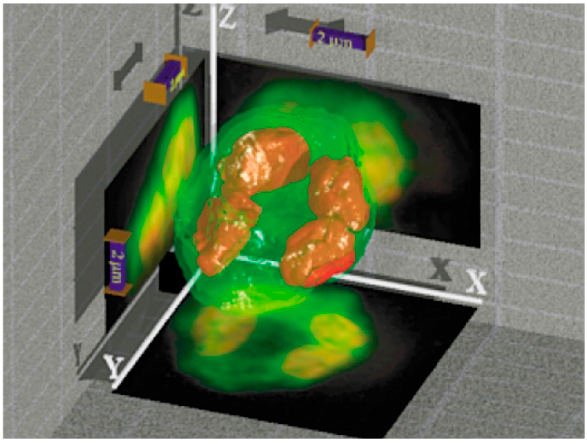
A surface-rendered version of a 3D reconstructed object. A moss spore (Polytrichum commune) was imaged by axial tomography, and a 3D representation was reconstructed. The entire diameter of the spore was below 7 µm (see scale bar: 2 µm). An overlay of the two detected fluorescence intensities is shown, and sum projections are displayed on the respective walls. From [42], with permission.
Figure 6.
A surface-rendered version of a 3D reconstructed object. A moss spore (Polytrichum commune) was imaged by axial tomography, and a 3D representation was reconstructed. The entire diameter of the spore was below 7 µm (see scale bar: 2 µm). An overlay of the two detected fluorescence intensities is shown, and sum projections are displayed on the respective walls. From [42], with permission.

Figure 7.
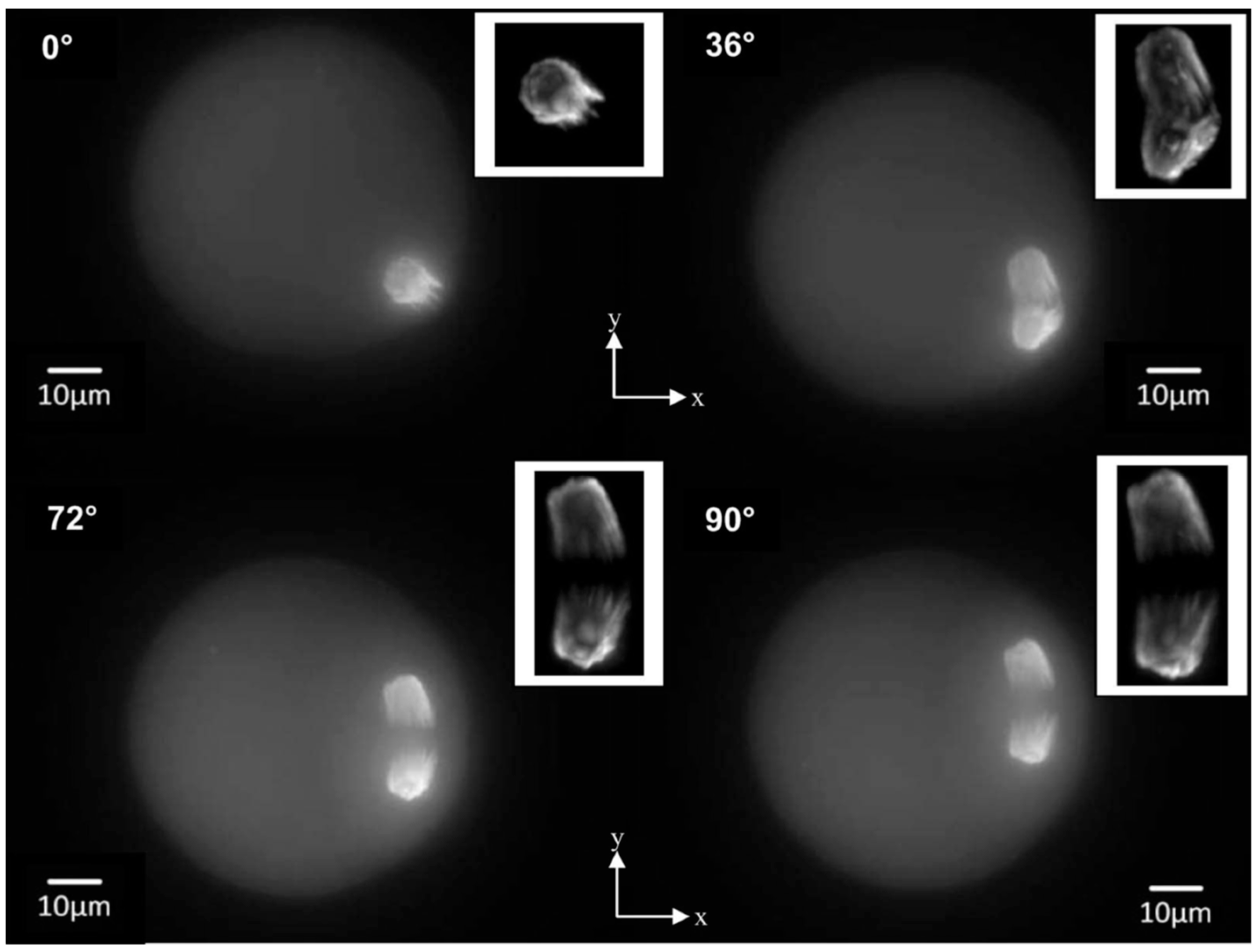
Axial tomography of a single mouse oocyte. Sum images along the optical axis of image stacks were acquired at 0°, 36°, 72°, and 90° rotation angles with a 63×/1.4 (oil) objective lens. The oocytes were fixed at the metaphase II stage, and the TACC3 protein associated with the spindle apparatus was visualized using rabbit anti-TACC3 and fluorophore-labeled goat anti-rabbit IgG antibodies. Insets: Deconvolution images of the spindle apparatus; cuts from the rotation series at the respective angles were deconvoluted using a Huygens software package. From [65], with permission.
Figure 7.
Axial tomography of a single mouse oocyte. Sum images along the optical axis of image stacks were acquired at 0°, 36°, 72°, and 90° rotation angles with a 63×/1.4 (oil) objective lens. The oocytes were fixed at the metaphase II stage, and the TACC3 protein associated with the spindle apparatus was visualized using rabbit anti-TACC3 and fluorophore-labeled goat anti-rabbit IgG antibodies. Insets: Deconvolution images of the spindle apparatus; cuts from the rotation series at the respective angles were deconvoluted using a Huygens software package. From [65], with permission.

Figure 8.
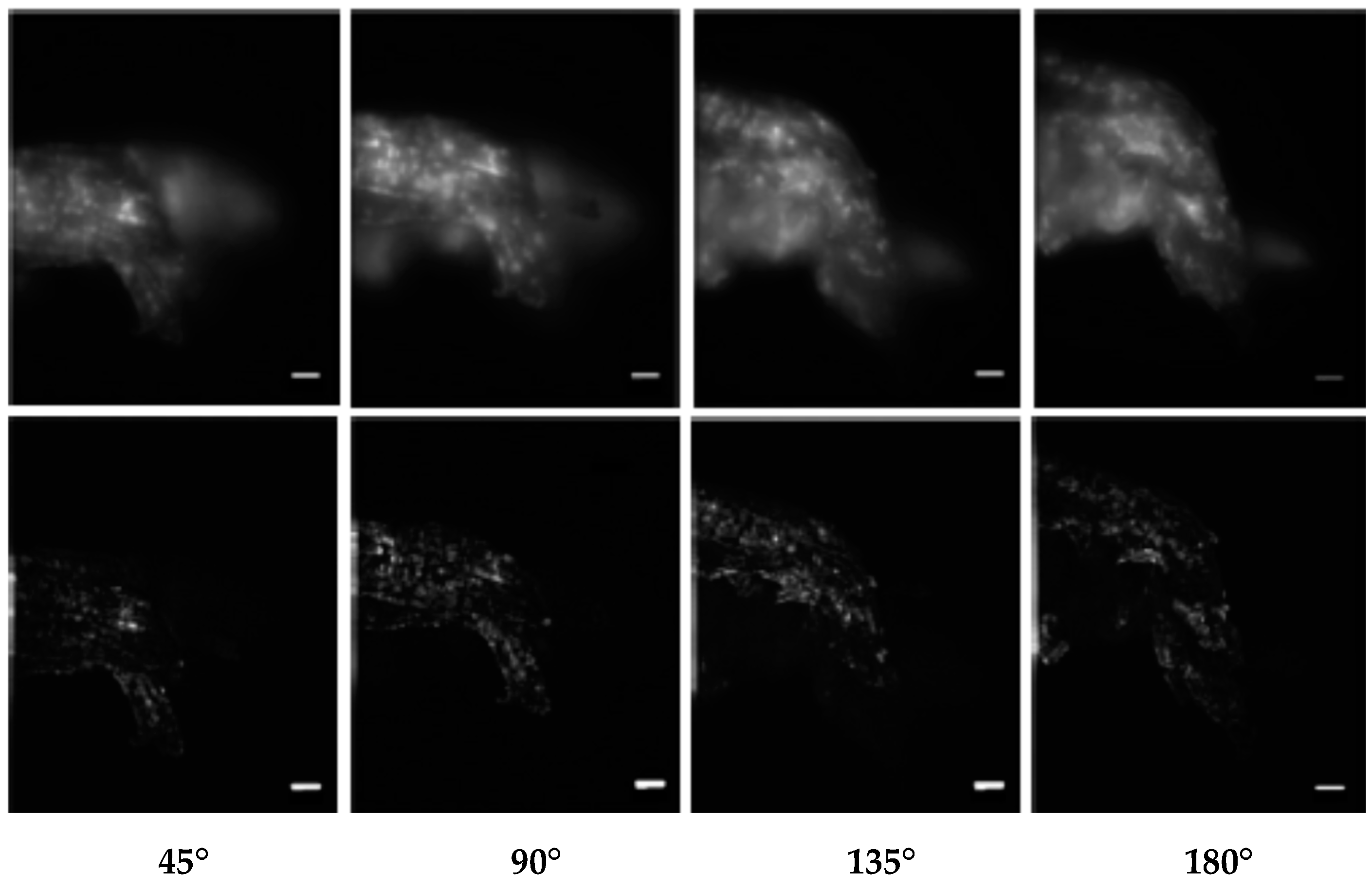
Combination of axial tomography microscopy and SIM (scale bar = 10 µm); upper row: Wide-Field (WF) microscopy images (AN = 0.25, working distance = 1 mm, λex = 671 nm) of autofluorescent structures in a cell of Cedrus deodora, registered at various rotation angles (45°–180°); lower row: the same cell registered by axial tomography with SIM under the same conditions. From [82] after modification.
Figure 8.
Combination of axial tomography microscopy and SIM (scale bar = 10 µm); upper row: Wide-Field (WF) microscopy images (AN = 0.25, working distance = 1 mm, λex = 671 nm) of autofluorescent structures in a cell of Cedrus deodora, registered at various rotation angles (45°–180°); lower row: the same cell registered by axial tomography with SIM under the same conditions. From [82] after modification.

Disclaimer/Publisher’s Note: The statements, opinions and data contained in all publications are solely those of the individual author(s) and contributor(s) and not of MDPI and/or the editor(s). MDPI and/or the editor(s) disclaim responsibility for any injury to people or property resulting from any ideas, methods, instructions or products referred to in the content. |
© 2024 by the authors. Licensee MDPI, Basel, Switzerland. This article is an open access article distributed under the terms and conditions of the Creative Commons Attribution (CC BY) license (https://creativecommons.org/licenses/by/4.0/).
Share and Cite
MDPI and ACS Style
Schneckenburger, H.; Cremer, C. Axial Tomography in Live Cell Microscopy. Biophysica 2024, 4, 142-157. https://doi.org/10.3390/biophysica4020010
AMA Style
Schneckenburger H, Cremer C. Axial Tomography in Live Cell Microscopy. Biophysica. 2024; 4(2):142-157. https://doi.org/10.3390/biophysica4020010
Chicago/Turabian StyleSchneckenburger, Herbert, and Christoph Cremer. 2024. "Axial Tomography in Live Cell Microscopy" Biophysica 4, no. 2: 142-157. https://doi.org/10.3390/biophysica4020010